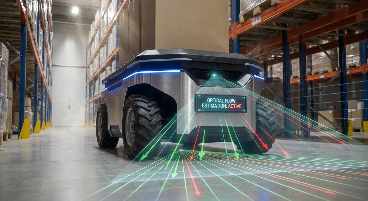
Optical Flow Estimation
Get dead-on navigation without GPS or beacons. Optical Flow Estimation spots motion between frames, letting AGVs gauge speed and dodge stuff in signal-dead zones.
Core Concepts
Brightness Constancy
The key idea: a pixel's brightness stays steady frame-to-frame, even as things move.
Sparse vs. Dense Flow
Sparse flow (Lucas-Kanade) chases key features; dense (Farneback) crunches vectors for every pixel.
The Aperture Problem
The aperture problem: a small window on a moving edge can't nail the true direction without wider context.
Spatial Smoothness
Smoothness constraint in dense flow: nearby pixels usually move together as part of the same thing.
Pyramidal Implementation
Multi-scale pyramids process images at different resolutions to catch big shifts that single-scale misses.
Motion Vectors
The endgame: flow fields as arrows or colors showing speed and direction for every point.
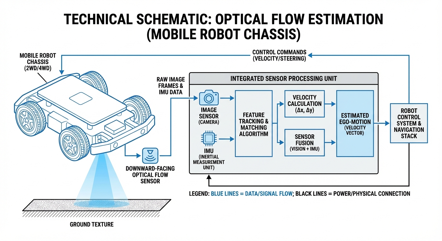
How It Works
Optical flow compares back-to-back frames from the robot's camera, tracking corners/edges or pixel patches to see where stuff shifted from frame t to t+1.
Solving $I_x u + I_y v + I_t = 0$ gives velocity (u,v). Paired with camera specs, it estimates the robot's 3D motion over the ground.
It's like a visual speedometer for the nav stack. No slip errors like wheel odometers—just pure ground-truth motion.
Real-World Applications
Visual Odometry (VO)
Warehouse AGVs use it to track position under cover. Integrate those flow vectors over time for precise trajectory estimates.
Obstacle Avoidance
Mobile robots rely on 'Time-to-Collision' from optical flow expansion. When objects rush closer, they quickly expand across the visual field, automatically triggering the brakes.
Precision Docking
Crucial for AMR charging stations. Optical flow lets the robot fine-tune its speed and direction for a perfect lineup with the charging contacts.
Slip Detection
By cross-checking wheel encoder data against optical flow visuals, robots spot when wheels are slipping on slick surfaces like oil or water and tweak traction control on the fly.
Frequently Asked Questions
What's the difference between Optical Flow and Visual SLAM?
Optical flow focuses on estimating speed and motion from one frame to the next (short-term stuff). Visual SLAM builds on that motion data but throws in loop closure and map-building to track position over long hauls.
Does Optical Flow work in the dark?
Standard optical flow needs visible light, so it flops in total darkness. Robots get around this with IR cameras or structured light projectors that add texture in dim spots, keeping the algorithm humming.
Why does Optical Flow fail on white walls?
This is the classic 'textureless surface' issue. Optical flow craves distinct features like corners, grains, or patterns to track movement. A smooth white wall? All pixels look the same—no way to measure shift.
How does wheel slip affect Optical Flow?
Usually not; that's optical flow's big win. It tracks the floor directly for true movement. Wheels spinning on ice? Encoders say you're moving, but optical flow says 'hold up, zero speed.'
What is the computational cost of Optical Flow?
Dense optical flow guzzles compute power and often needs GPU boosts like NVIDIA Jetson. Sparse optical flow, tracking just key points, is lightweight and runs fine on basic microcontrollers or modest CPUs.
Is a Global Shutter camera required?
Absolutely, it's a must. Rolling shutter cameras grab lines one by one, creating wobbly 'jelly' effects in fast motion. That warps the image and throws off flow calculations big time.
How do dynamic objects (people) affect the reading?
Moving objects mess with the algorithm since it assumes a static world. Smarter versions use RANSAC or IMU fusion to ditch 'outlier' vectors from people walking by, zeroing in on the steady background.
What is the difference between Lucas-Kanade and Farneback?
Lucas-Kanade is a sparse approach that assumes steady flow nearby, so it's quick and great for tracking corners. Farneback goes dense, calculating flow for every pixel to build detailed motion maps—but it needs more horsepower.
Can deep learning replace traditional algorithms?
Yep, networks like FlowNet and RAFT lead the pack for spot-on accuracy and toughness in tricky light. Downside? They demand way more hardware than old-school geometric methods.
How does height affect Optical Flow accuracy?
Optical flow tracks pixel speed, which ties to depth. For real-world speed in meters per second, you need exact floor distance (height). Bumpy floors or camera tilt? Hello, scale errors.
What is the ideal frame rate for Optical Flow?
Higher frame rates are better—they cut frame-to-frame shifts. Fast AGVs love 60fps or more so features don't leap too far, fitting the 'small motion' rule most algorithms expect.